

Visualizing Antenna Fields

[October 2020] Computers have come a long way in the past 40 years. Interactive applications can show quite a bit about how an antenna will perform. Yet, real world measurements and field checks can sometimes provide a surprise or two.
Learning more and being able to visualize how antennas radiate can go a long way to helping the engineer understand the how the antenna works.
It has been 30 years since this paper originally was written and delivered at an SBE Engineering Conference. Much pondering has occurred since then, wondering whether the theory put forth is correct or not. I continue to believe it is correct, primarily because of two things:
1. The First Law of Thermodynamics is also the Law of Conservation of Energy. It states that we may neither create nor destroy energy. We can only change its form. Because all electromagnetic radiation is composed of photons, we cannot simply cancel them or make them disappear.
2. If, in an experiment, we:
- place two transmit antennas some distance apart and then off to one side,
- set up a receive antenna so that the two signals from the transmit antennas arrives at it simultaneously,
- and adjust the phasing and amplitude of the two transmit antennas so that their two signals arrive at the receive antenna with precisely the same amplitude – but exactly 180 degrees out of phase…
… the output from the receive antenna will be zero.
We say that they have “cancelled,” and so they have. Apparently, there is “no radio signal in the area.” Yet, the two fields from the transmit antennas are still alive and well, and are propagating at full strength right past the receive antenna.
Another example: it is simplistic to state there is very little field from the back side of a Yagi-Uda antenna because they cancel. A multitude of fields are there, contributed by each of the elements of this antenna. They are merely out of phase and sum up to a small value within the receiving antenna of a field intensity meter.
If we can visualize the experiment and underlying physics, an understanding of Electromagnetic (EM) propagation is within our grasp.
It is hoped that this brief discussion will lead to a discussion of the topic among broadcast engineers and others interested in Electromagnetic (EM) propagation. We now return you to my original thoughts, as presented in 1988:
Rooted in Theory
The method of visualizing antenna fields as presented here must be categorized as theoretical because as of yet, instruments are not available to provide direct observations.
It has been said that the reason mankind has made so much progress in science over the last century is due to learning to make accurate instruments, rather than improved imagination techniques. But the following will require that you exercise your imagination because the instrument to do the observation has not yet been invented.
Perhaps your imagination will be challenged into thinking about such an instrument by what follows.
Multi-Element Antennas
Directional antennas have been in common use for more than a half century protecting some AM stations from interference and allowing FM and TV stations to increase their effective radiated power to many times the transmitter output power.
Additionally, the low output power of translators, STL transmitters and the like may be effectively multiplied with so-called “gain antennas” to put a stronger signal over populated areas, or into another gain antenna which is the target.
All these antennas can be classified as “multi-element” antennas, but what is most important to us is the electrical result – which is that they are “multi-field” antennas.
However, when we look at the graphic representation of the pattern of an antenna, it must be remembered that this is not the real radiation from a multi–element antenna, but the effective resultant.
The real radiation is a set of fields, one from each element of the antenna. This is the case whether it be an AM directional antenna, an FM or TV multiple bay antenna, a Yagi, or any other antenna composed of multiple elements or multiple conductors.
The effective fields may be derived mathematically and measured with a field intensity meter (FIM), but the most important device in the process is, of all things, the receiving antenna.
This simple device – whether the loop built into the lid of a FIM or just an old coat-hanger stuck into the broken off stub of a car radio socket – the radio antenna becomes an integrating device, transducing the many fields it intercepts into a resultant electrical current which is conducted to the input of the receiver or meter to which it is attached.
Were it not for this integration of all the currents in the passive receiving antenna, all the efforts of the design engineers would be in vain.
Nevertheless, bear in mind that any antenna is intercepting not only the fields of the station to which it is tuned, but to all the other fields that are found in its environment: all the broadcast and communication signals, short wave, VLF, VHF, UHF, noise and whatever might be arriving from outer space. All of these fields are transduced into electric currents based on their EM field intensities and phase relationships, so the resultant at the antenna terminal may be a complex mess.
Analysis and Evaluation
In order to understand how such a multi-field set is generated, we must select a single frequency and design a simple system that will generate a simple set of fields so that it may be evaluated. The same principles will apply whether the antenna is composed of elements in a vertical stack or an array of towers spread across a cow pasture.
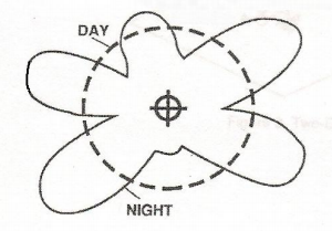
Figure 1 – The Effective Field of an AM Directional Antenna
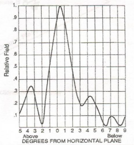
Figure 2 – Effective Field of a Vertically Stacked Antenna
Figure 1 is the effective field of an AM directional antenna – but this is not the real field. Figure 2 is the effective field of a vertically stacked FM, TV, or communications antenna – but, again, this is not the real field.
To get an understanding of how all this comes about, a simple two-element AM antenna will be analyzed. Its parameters are:
1. Spacing: 180 electrical degrees.
2. Phasing: 0 electrical degrees (that is, the two elements are driven in phase with each other).
3. Power ratio: 1:1 (each element receives the same amount of RF power).
4. Element height: 90 electrical degrees vertically polarized.
5. Antenna orientation: 0 degrees true (N-S).
We can represent this antenna graphically in this manner:
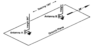
Figure 3 – A Two-Element AM Directional Array
Note: A simple way to determine the approximate length of an electrical degree in feet is to divide 2733 by the frequency in kHz. To determine the length in meters, divide 833 by the frequency in kHz. If you want to calculate in MHz, just move the decimal point to the left three places (2.733 or 0.833). Then, if appropriate, apply the velocity factor.
The Effective Field
Fig. 4 shows the resultant effective field of this configuration. To the North and South are nulls, while to the East and West, lobes are seen.
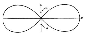
Figure 4 – The Effective Field of a Two-Element Array
But if this does not represent the real fields, how is it derived? Again, by integration in the receiving antenna.
The real fields shown in Fig. 5 expand as big circles, so the nulls in the North-South directions are just as strong as the lobes.
![]()
Figure 5 – Actual emitted fields from the transmit antennas (N-S displacement exaggerated)
The way to understand this is to note that, because of the 180 degree spacing between the transmitting elements, the field from the South element, for example, arrives at a receiving point on the North radial later than the field from the North element.
The receiving antenna located out on the North radial is an energy transducer, so while the EM field from the North element is trying to induce current upward in it, the EM field from the South element – having a 180 degree phase relationship with the North element due to the time delay caused by the spacing – tries to induce current downward in it.
The result is that the two equal but opposite currents effectively cancel each other, so the resultant current to the receiver is zero. Both the EM fields are still there at full strength but the receiving antenna has, because of the phase relationships, integrated their effects resulting in its terminal output voltage and current to be zero (or nearly zero) in this direction.
Effective Gain
Another look at Figure 4 shows that the lobes in the East-West directions extend farther than would the signal from a single element with the same RF power.
In these directions, the two EM fields from the elements arrive at the receiving antenna in phase. Some energy from each field is transduced into an RF current based on its strength, but the receiving antenna again integrates them into a single current to the receiver input. This stronger signal is a result of the effective field gain, the understanding of which is crucial to the evaluation of a directional antenna system, whether AM, FM, TV or any other application of a multi-field antenna.
So far, the shape of the effective field between the compass points has been ignored, but it will be noted that the curve representing field strength diminishes as it moves away from the E-W radials toward the N-S radials. This is a result of the timing of the arrivals of the two EM fields at a particular azimuth. This timing is expressed in electrical degrees, rather than in real time.
It can be seen that in the E-W azimuth the phase relationship between the two fields is zero and increases to 180 degrees as we rotate toward the N-S azimuth. This simply represents the electrical time relationship between the two EM fields. To determine or predict the field intensity at any azimuth, a triangle can be calculated and trigonometry applied to determine the value. It can also be expressed using vectors.
Note in Fig. 6 that if the angle becomes 180 degrees, the effective voltage line (Eeff) diminishes to zero.
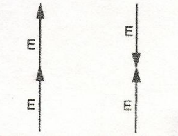
Figure 6a Field Vectors in Field Vectors in E-W Directions; if N-S Directions; if each vector has a each vector has a value of E, the value of E, the result is 2E result is zero
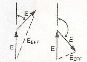
Figure 6b Examples of Field Vectors between the N-S and E-W directions. The effective field is represented by the dashed line; the angles shown represent the phase angle values
Furthermore, if different elements within the antenna are fed with different power levels, the vector lengths representing field intensity are proportional to the power levels. Both the angle and the length of the vectors determine the value of the effective voltage (Eeff).
From all this, you can see that if an engineer stands in a null (minima) of a DA pattern and measures a very small value of field intensity, he is standing in a complex set of fields, one from each element of the array, each of which is still at its full strength based on the distance from the elements and the power fed to each of them.
The antenna of the field intensity meter (FIM) integrates the set of fields based on their relative amplitudes and phases and the meter indicates a value that we call effective field intensity.
Effective Radiated Power (ERP) For FM and TV Antennas
Effective radiated power and effective field intensity are directly related. Each bay of an FM or TV antenna is an antenna element just as are the individual towers of an AM directional array. The pattern from a single bay is similar to the textbook pattern of a vertical dipole. It may be modified by the mechanical geometry of the antenna or dual polarization, but it still is more or less the classic toroidal or doughnut shape.
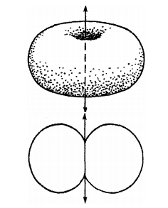
Figure 7 – Field from a single vertically polarized FM antenna. The arrows represent the antenna axis, or direction of the dipole element
If two or more bays are “stacked” in a vertical plane, they become a collinear array. Collinear is a mathematical term which means “sharing the same line” and in this case the line is vertical. As in the E-W directions of the AM antenna previously described, the field from each element induces or transduces a current into the receiving antenna.
Therefore, the effective field from a twelve-bay FM antenna, for example, is composed of 12 separate fields that induce 12 separate currents into the receiving antenna, which are then integrated into a single current which goes to the input of a receiver.
Again, this is the effective field and not the real radiation. The real radiation consists of 12 doughnuts leaving the 12 bays simultaneously.
The pattern of such a twelve-bay antenna will be seen to have a lot of little lobes and nulls in it unless null fill is incorporated in the design. Null fill is accomplished by manipulating the set of real fields to modify the effective field or pattern.
Unmeasurable Fields
The conventional field intensity meter cannot measure the real fields, but only the effective resultant field.
The standards of the non-ionizing radiation rules are often based on measurements taken with field intensity instruments, but from the previous discussion, it can be seen that a person could be in powerful EM fields that would not be indicated on the meter.
So are measurements taken by this method adequate to determine the hazards, whether real or imaginary, from non-ionizing radiation? If there is danger from this source, it may be more complex than just the simple integration of induced electric currents. It could be presumptuous to come to such a conclusion.
Measurement of Multi-Field Energy in Null Areas
One may be led to conclude that EM field measurements would be impossible within the null areas of a pattern. Nevertheless, the issue should be addressed with an open mind to try to determine whether it might be possible.
Bear in mind that receiving antennas as we know them are, regardless of their mechanical complexity, passive devices with the function of intercepting an EM field, extracting a bit of energy from it and transducing this energy into an electrical current which is then transmitted to the input terminals of a receiver or instrument.
Would it be possible to select only one field from the multi-field set to measure it or detect the intelligence with which it has been modulated?
If such a device could be developed it could be extremely valuable and have many applications. Some examples are:
1) A synchronous AM transmitter location within a null of the station could receive the signal directly, process it and then re-transmit it, assuming the re-transmitted signal could be kept out of the received signal.
2) Since we have developed the method of “nulling out” signals so that they are not received by conventional methods, a system of secret communications could be developed for government and military applications. Who knows? This may have already been done.
3) In scientific research, it would make for interesting listening to radio signals from space. It is remotely possible that such multi-field sets are arriving on earth out of phase so that they cannot be detected by conventional methods.
Such a device might be a variation of current antenna technology or it might be radically different. Rather than being a passive device, it might have to be active. It might employ some variation of quadrature detection to separate the energies extracted from the EM field set.
It is easy to say such an accomplishment is impossible. That has been said many times before about machines and devices no one previously had even dreamed of. It certainly seems to at least be worthy of consideration.
Anti-Skywave Antennas
A great deal of attention has been given to anti-skywave antennas recently.
This is because more than 4,500 AM stations share only l17 channels in this country – not to mention many more stations outside its borders – but still having the capacity to reach into the US at night, causing further interference. If we could somehow effectively eliminate the so-called skywave radiation that goes up and reflects off the ionosphere and then comes down hundreds or thousands of miles away, interference would be greatly reduced and local and regional stations would have much improved coverage areas at night.
Depending on its electrical height, a conventional AM antenna transmits an edge sliced, half-bagel shaped signal rather than the doughnut of FM and TV (Figure 7). Part of the signal travels along the earth’s surface, but part of it travels at upward angles – and this is the culprit of skywave. If we could electrically step on the bagel, squashing it out flat, the problem would be solved. We cannot do that, but we can attempt to effectively flatten it with multi-field energy.
The problem is to transmit fields which are in phase in the ground wave component, but which will arrive out of phase in the skywave component. The reflected skywave fields must arrive back at the earth with equal strength and 180 degrees out of phase, or as closely as possible to these parameters.
This defines the challenge to anyone who would design such an antenna.
As the height of the ionosphere varies and it “bends” the skywave back toward the earth rather than reflecting it as a mirror, it is not possible to select a precise angle at which the arriving fields will satisfy these parameters. A further complication is the possibility that giant waves or undulations in the ionosphere constantly change the angles of reflection. This is evidenced by the regular “fade in, fade out” effect at certain times from distant AM stations.
If this is the case, then it means than the reflection angle is constantly changing at the frequency of the undulations. All in all, it is not an easy problem with easy solutions.
Multi-Field Radiation From Multi-Conductor Antennas
Although there may be disagreement on this theory, it should be considered that the possibility exists that each wire or conductor in a multi-conductor antenna generates its own EM field.
Even though they are usually only from one to five electrical degrees away from each other, and are often connected together somehow, each wire may be considered as a separate radiator, generating its own half-bagel shaped field. At a distance, the phase difference from the separate fields is so small that normally there are no significant directional effects. Due to the close proximity, the separate fields may perhaps “meld” into a single EM field, but even if this is so, viewing the fields as being separate may help in the analysis and evaluation of the distant effective field.
Mutual impedance might be considered a result of the parasitic effect in that besides the power being fed into the input of one wire radiator, the very near field of another wire radiator attempts to induce a current into it with a different phase relationship and causes the effect known as mutual impedance. The farther apart that the radiating elements are from each other, the less is this effect, so at distances from one to five degrees the effect is very great.
Even with this effect, each radiating element may still be considered separately for analysis of antenna performance. From this perspective, it can be seen that the resultant input impedance of such an antenna may be manipulated to vary the values of resistance and reactance for best impedance matching.
The Receiving Antenna
Applying the law of reciprocity, the multi-element receiving antenna can be evaluated the same as a multi-element transmitting antenna.
Considering a single arriving EM field from any specified direction, each element – parasitics included – will transduce some energy from the EM field to current and then re-radiate it. If, as in the case of a Yagi antenna, the original field and all the generated fields from the parasitic, elements arrive approximately in phase (or multiples of 360 degrees), effective gain will be realized when all the induced currents are integrated in the driven element.
This principle applies even in the case of an antenna where all elements are driven, such as an AM array. If the transmitting pattern indicates a strong lobe in a particular direction, then the array will perform well as a receiving antenna in this direction.
For a complex analysis, imagine the ten fields from a ten-element VHF Yagi antenna arriving at another ten-element Yagi. Each of the ten transmitted fields will transduce a bit of energy into each of the parasitic elements of the receive Yagi, which will re-radiate small fields.
Each of these re-fields, with a phase lag in them, will then arrive at the driven element in a multiple of 360 degrees with the ten original transmitted fields.
How many fields will ultimately transduce energy into the driven element? A lot. It would take a mathematician to determine the full number.
Conclusion
The ultimate performance of any multi-element antenna must be evaluated by the sum total of all the integrated currents at the output terminal of the receiving antenna at a distance, whether single or multi-element.
The main concern is, of course, is how much voltage (or current) will be present at the output terminal of the receiving antenna, whether AM, FM, TV or otherwise.
In the case of multi-field transmitting antennas, this value is always the result of not the intensities of the real fields, but the combination of all the field intensities and their phase or timing relationships. Multi-element receiving antennas perform based on the same criteria. By proper design, the value of receiving antenna terminal voltage or current can be increased or decreased, within limits, at will to attain the result desired.
When evaluating the performance of any multi-field antenna, try to visualize the field traveling outward in a circle from each element, based on its amplitude and phase or timing. What is important are these relationships when they arrive at a receiving antenna, whether for entertainment, communications or scientific reasons. The receiving antenna is the integrating energy transducer that is all important.
– – –
The late Ron Nott was a long experience electrical and electronic engineer, and the Founder of Nott Ltd. (NottLtd.com), antenna specialists, located in Farmington, NM.