

Debunking Half-wave Antenna Myths

The half-wave vertical antenna is a popular configuration in the amateur radio community. Unfortunately its performance is too often compromised by a lack of ground or symmetrical counterpoise.
A battery-powered transceiver and antenna coupler sitting atop a table coupled to ground only through the capacitance between the equipment and the earth is a bad idea. This configuration can affect antenna gain, can be hazardous to your health, and creates risks for curious onlookers.
In my opinion there is a dearth of information within the amateur radio community regarding the very high levels of RF radiation that exist in typical Field Day camps, DX expedition sites and typical residential sites. Did you know that the electric field intensity two feet away from the halfwave antenna set up in Figure 1 exceeds the FCC maximum permissible CW exposure for the general public at a power output of only 25 Watts?
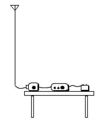
Would you think twice about sitting at that table if you were operating at a typical 100 Watts? I would think so. And, while people rarely are found sitting at a table at the base of a half-wave broadcast antenna, the information here is worth considering when calculating the level of RF exposure to which broadcast workers may be exposed.
Reference Point
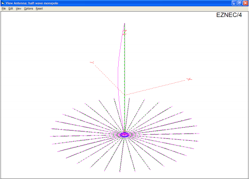
As a reference antenna, let us consider a permanent installation where 30 copper ground radials are buried 6 inches beneath 5 mS/m soil with epsilon of 13, as shown in Figure 2.
The vertical monopole is intended to operate as a quarter-wave antenna in the 40 meter band, and as a half-wave antenna in the 20 meter band. For our purposes, assume that the ground wires are each 20 feet long AWG 12, and the vertical wire is 34 feet of stranded AWG 16 hanging from a tall invisible tree.
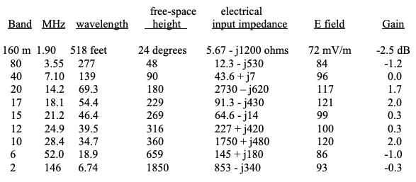
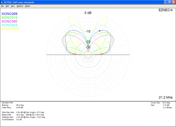
As seen in Table 1, the antenna’s expected input impedance at 7.1 MHz is 43.6 + j7 Ohms, and at 14.2 MHz is 2730 – j620 Ohms. In the table, the E field column refers to the vertically polarized electric sky-wave field intensity at one mile at an elevation angle of 20 degrees for 1000 Watts input to the antenna.5 The gain column is relative to the quarter-wave monopole electric field. The omni-directional far-field elevation patterns of Figure 3 are developed per NEC4.1 It is worth noting that the fields at 20 degrees elevation are not necessarily the maximum fields, especially at the higher frequencies. Of course the azimuthal or horizontal radiation pattern is omni-directional.
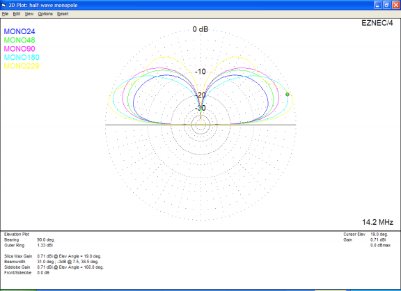
The collection of far-field elevation patterns in Figure 3 includes the typical electrical heights used in commercial AM broadcast installations. The most gain is had with a 5/8 wave tower, shown in yellow.
Electrically taller monopoles operating below 1800 kHz are usually too costly for commercial stations relying on ground-wave propagation, since the gain at low elevation angles decreases rapidly with heights greater than 225 degrees. The only reason for using a tower taller than this would be if the tower already existed, originally intended for some other purpose.
Some interesting multi-lobe patterns emerge at HF frequencies where physical height is not so much a concern, and electrical heights much greater than 5/8 wavelength are practical. If sky-wave propagation via ionospheric bending of electromagnetic signals is desired, a close study of Figure 4 is suggested.
A realistic maximum gain of 9.6 dBi can be obtained at 146 MHz with the 34 foot vertical sky-wire over 5 mS/m earth.4 If there were something that could reflect or refract this VHF signal launched at 69 degrees elevation, some interesting propagation could occur.
Drawbacks of Hasty Installation
Now let us consider the reality of a portable installation which has no ground radials either above or below the soil.
We can model a transceiver and external battery on a table as a five foot horizontal wire fed in the middle hovering three feet off ground. In order to keep the length of the vertical wire a half wave at 14.2 MHz, the skyhook must be raised three feet, to 37 feet off ground. The input impedance over 5 mS/m earth becomes 737 – j2840 Ohms, but nevertheless it is still easy to couple to the transceiver with a simple tuned transformer.
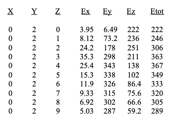
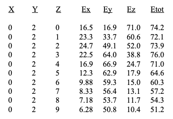
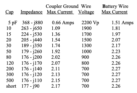
Even with this relatively short five foot connection to the base of the antenna, a significant amount of horizontally polarized electric field is radiated. That is why in Table 3 there are three E field columns, one for each axis. The common RF engineering practice is to measure electric fields in root-mean-square Volts per meter, and electric potentials that can create corona or arcing in peak volts. Note that all field values in Table 3 are reduced to ten percent of the tabular values if only ten Watts of RF is delivered to the antenna, instead of 1000 Watts.
It is important to consider the high RF voltage present at the operator location, and the relatively high radiated electric field near the bottom of the antenna.6 The fact is that the operator is a closely coupled part of the RF circuit in this case, and therefore low transmitter output levels are advised, unless the operator wants to risk cooking himself.
At a minimum, the operator should wear shoes with insulated soles, and not sit on an aluminum lawn chair. Otherwise every time the operator shifts position he may see a change in SWR, which can be quite annoying. Onlookers standing near the antenna will also perturb its performance, and are in danger of receiving a nasty RF burn if they touch any part of the circuit.
General Public RF Exposure Limits
According to the FCC Rules, the maximum permissible electric field exposure for the general public is 824/f Volts per meter for 1.34 < f < 30.00 MHz. Thus the limit when operating at 14.2 MHz is about 59 V/m. Table 2 is obtained for the case of an invisible observer standing two feet North of the antenna (in the Y direction). The 367 V/m at a height of four feet above ground egregiously violates the limit, and exposes the operator to a $10,000 fine.
If CW power is reduced below about 25 Watts, the danger is reduced to acceptable limits. Keep in mind that the effective field intensity will be greater if some form of modulation other than plain on/off keying is used, such as AM or SSB. As you know, more power is delivered to the antenna when sideband energy is added to the equation. You may want to just limit your operation to QRP, and be done with it! And yet we still do not understand the long-term exposure risks in terms of increased chance of developing brain cancer, etc. Personally I know of far too many cases of cancer within the ranks of professionals chronically exposed to high levels of HF radiation.
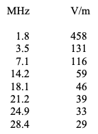
Let me point out that Table 3 lists the threat at 14.2 MHz only. In fact the near field intensity from this 37-foot tall wire at lower ham radio frequencies is even greater, because the RF voltage at the base of the antenna is higher than the 20 meter band value.
For example, the base input voltage at 1.9 MHz is 38 times higher, per Table 5. Did you think this antenna would be close to resonance at 7.1 MHz where the wire is a quarter-wave long? This would only occur if we were working against a reasonable ground system.
We can reduce the RF near-field intensity by adding some ground stakes beneath the equipment per Figure 8. Table 4 lists the 14.2 MHz RMS electric fields that a person would encounter when standing two feet North of the vertical wire. The exposure still exceeds the FCC maximum when operating at 1000 Watts, but now the power only needs to be reduced to 600 Watts in order to fall into compliance.
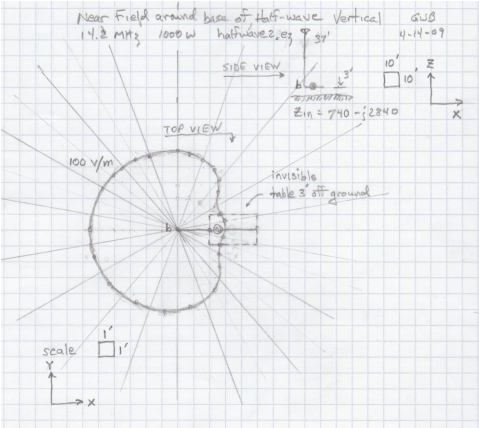
Figure 5 – Sketch of 100 V/m contour, no ground stakesThe 100 V/m contour around the base of the antenna for 1000 Watts delivered in Figure 5 tells us that there is a large hazardous area that would have to be roped off to prevent the general public from excess exposure. If power were reduced to 350 Watts, the maximum limit of 59 V/m would follow the contour shown above.
If wood stakes are placed in a 12 by 14 foot rectangle, and ribbon strung between these stakes, the ham radio operator has co-opted close to 170 square feet. This does not include his seating, sleeping and equipment areas. In a crowded field-day exercise space is often limited.
We can model a worst-case onlooker as a six foot metal post erected close to the vertical wire standing on 100 pF tennis shoes.3 When the onlooker stands five feet away, the 14.2 MHz impedance becomes 733 – j2810 Ohms, the RF current through the onlooker’s feet totals 185 mA, and the voltage across the soles of his shoes is 29 peak Volts.
Danger!
If however the onlooker moved to the end of the table and touched a battery post, his skin would fry and the antenna input impedance would stabilize at 794 – j1250 Ohms, the onlooker’s feet would experience 923 mA, and the shoes would see 146 peak Volts. This is a massive change to the operating conditions.
Therefore I highly recommend that the hasty operator stake off his area with some yellow tape printed in big bold letters saying “CRIME SCENE – DO NOT CROSS.” The point being: this is not a joking matter.
As an alternative, the installation can be fitted with a short ground rod attached to the negative terminal of the battery.
If a 12-inch long copper rod is stabbed into the dirt below the battery and a three-foot cable run from that to the battery post, the antenna input impedance becomes 836 – j1360 Ohms, and the danger to the operator is significantly reduced, as long as he stays close to the ground wire.
In either case, equipment grounded or not, the dangerous area near the bottom of the vertical wire needs to be cordoned off.
Also note that the high reactance of the floating configuration has been cut in half, so impedance matching to 50 Ohms becomes easier. A simple RF transformer can be used to reduce the impedance to a value within the range of a typical coupler.
Such a transformer also serves to reduce the possibility that the operator will accidentally touch the high voltage present at the bottom end of the antenna wire. A second ground stake driven into the dirt at the other end of the table with a wire attached to the couplers metal case will serve to improve safety even more. If your coupler has a plastic case, I hope you are operating QRP only.
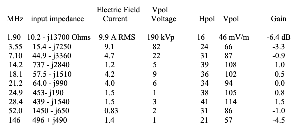
Table 5 – Antenna Performance with only a short floating counterpoise wireObviously the base voltages at the lower frequencies are completely untenable even at QRP power levels. The losses in the coupler are likely to be huge, so even if the voltage could be withstood by the insulation, the couplers internal components may overheat. An RF transformer would reduce both the resistance and reactance of the antenna input impedance, so there is not much to be gained with a transformer when operating at the lower frequencies. Top-loading or a longer wire would help.
Interesting Elevation Patterns
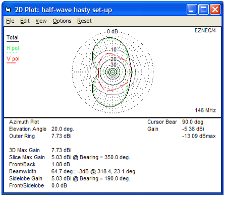
Another problem with this particular short, asymmetrical counterpoise feed attached to a 34-foot wire, is the change in radiation patterns at VHF. Not significant at HF frequencies, but per Figures 6 and 7 the two meter band performance is clearly disturbed.
Operating such a wacky antenna in the two meter band would be an adventure, but that is perhaps what ham radio is all about. The most important caveat about operating these floating antennas is safety. It may seem obvious, but I would be derelict if I did not state that you should always begin a new operation at low power.
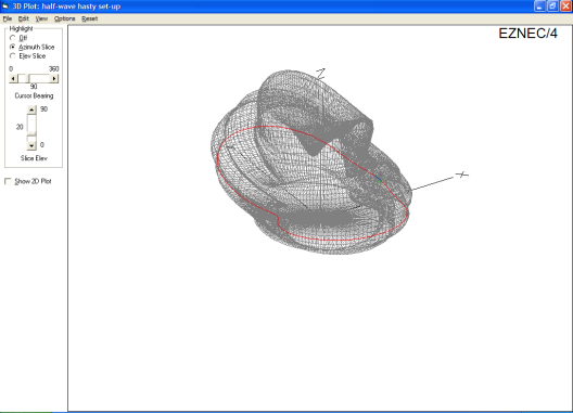
The three-dimensional radiation pattern of Figure 6 shows the total E-field, and does not separate the horizontally-polarized field from the vertically-polarized field shapes at 146 MHz. Figure 7 shows the Hpol and Vpol fields individually, and the different pattern shapes that can be expected on the horizontal plane at a 20 degree elevation from the transmitting site. As you can see, these two patterns differ substantially, with a strong null in the Hpol pattern to East and West, off the ends of the short horizontal wire lying atop the table.
Adding Small Ground Stakes
If we drive a 12 inch galvanized nail into the dirt at each end of the table, and run a wire up to the negative battery terminal, and another up to the ground side of the coupler, we can tune the antenna impedance with a high-Q shunt capacitor. Keep in mind that these ground wires have a lot of inductive reactance at 14.2 MHz, so the coupler will not behave as ideal lumped-parameter circuit theory might lead us to believe.
There is also a lot of coupling between the wires around the equipment table, so tuning can be tricky and counter-intuitive.7
So we cannot pull the resistance down to 50 Ohms with a single shunt capacitor, because the overall reactance in the shunt leg of the circuit is controlled by the fixed amount of inductive reactance in the wire below the capacitor.
That is, we cannot obtain a capacitive reactance low enough to swamp the impedance adequately. Thus we will have to add some series inductance between the coupler and the antenna to bring its high negative reactance to a lower value. Or we can use an RF transformer instead.
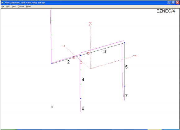
But if we place an inductor at the output of the coupler (wire 2 in Figure 8), nothing useful happens (strange, but true). The input impedance to the vertical wire as seen by a source located in wire 3 in Figure 8 between the battery and the coupler is 177 – j93 ohms with no series coil. We can tune out the reactance with a 1.04 micro-Henry coil, but a reasonably low impedance such as 177 – j93 Ohms is well within the range of most antenna couplers.
Conclusions
a) Some empirical data should be collected using modern and accurate instruments in order to settle the questions raised about impedance transformation in hot or floating antenna configurations, and the E-field intensities around them. There are many highly accurate, inexpensive field intensity meters available these days that are designed specifically to measure RF radiation exposure levels.
b) An RF transformer located at the base of a half-wave antenna is a practical means of reducing a high impedance to a lower impedance which is easier to match to 50 ohms. This can be modeled in NEC4 by using the NT card (see the NEC4 manual, which has an example).
c) Safety issues are paramount when considering a floating antenna installation, but are still a serious issue even when proper RF equipment grounding has been installed. –
Notes
- EZNEC/4 double-precision NEC4 version 3.0.59 with one-foot-long current elements below 30 MHz, and 6 inch long current elements above.
- See http://www.AA5TB.com/efha.html and related sites for some nice RF transformer antenna coupler designs using resonated primaries.
- Of course a human being is not a perfect conductor, and a better model of a person would include loads along the wires representing his arms, torso, head and legs. Still let us not forget that a salty, sweaty body in the summer sun conducts fairly well at RF, and the skin is likely to burn if enough current is applied even over a short period of time. If socks and shoes are also soaked in sweat, or worse yet the person is barefoot, beware indeed!
- Note that the unit called dBi is gain relative to a theoretical lossless isotropic radiator, and does not include earth losses. Thus 9.6 dBi for any single-element antenna close to real earth is impresssive. Compare this figure to the 0.7 dBi of our half-wave vertical antenna, which is almost a 9 dB increase. Again, ground-wave propagation comparisons are completely different.
- One kilowatt of power is a standard used in the FCC figures of Part 73 of the Rules and Regulations relating to electromagnetic radiation from broadcast antennas. This 1000 Watts is the familiar and usual value used to compare antenna performance in the professional broadcast community, although it is typically the upper limit within the amateur radio community.
- The FCC publication, A Local Government Officials Guide to Transmitting Antenna RF Emission Safety: Rules, Procedures, and Practical Guidance, is available at www.FCC.gov. Please note that the imposed limits assume a CW source, and that the effective fields will be higher if SSB or AM are used. Thus when operating in these modes, it is a good idea to reduce transmitter carrier power to about 80 percent of the CW values listed in the report to ensure compliance.
- Keep in mind that NEC does not behave well when electrically-small closed loops are part of the wire configuration. Since we are modeling over real ground, and not tying any of our equipment ground wires into a buried radial ground system, this takes one leg of a possible closed loop out of the picture.
– – –
Grant Bingeman, P.E., is a design engineer, well-known in the broadcast industry for his work at Gates/Harris, Rockwell/Collins, and Continental Electronics. His email is GrantBingeman@cs.com Or, visit his website is at http://www.km5kg.com/ for more articles and software downloads.